

As investors, we are looking to preserve our capital as our first goal. The key is - we NEED the capital to make profits. No capital - NO gains. So making a profit is only the second objection of investing.
As a simple example - with $1M we need only 5% to make $50k. While if we lost 90% of the value - which has happened to technology stocks in the early 2000s during the dot com bubble crisis - then we’d need to make 50% to achieve the same profit of $50k which is MUCH harder to do in a manageable, maintainable and consistent way.
In this article, we are going to:
- learn about tactical assets allocation and how it helps to reduce risks
- see how we can assess risks quantitatively
- discuss 3rd party results of a strategy backtest
- build a similar backtest using Yahoo Finance data and Python data science toolkit
Adding such an assessment to your personal strategy evaluation pipeline could help to make a better (quantitative) decision for using one strategy over the other. Or at least to discard some of the ideas and strategies with poor performance at the early stage.
Tactical asset allocation (TAA)
So what do we do to protect ourselves from losses? - We reduce RISK.
The risk in investing is traditionally measured by historical volatility and drawdown of the portfolio. So ideally we want a strategy with the highest returns and the lowest volatility and drawdown.
Have you ever heard of the 60/40 strategy where you invest 60% money in bonds and 40% in stocks and maintain the balance over time? What we do is try to reduce the risk of stocks market volatility by holding bonds.
One thing to understand is that is not a 100% passive investment - you will need to look at the market periodically and rebalance the portfolio accordingly to the updated economic conditions.
Using bonds protects us around periods of high interest rates. When interest rates are high more investors tend to buy bonds rather than stocks. Because bonds start to generate good returns with much less risk (volatility). On the other hand when interest rates are low - bonds are not as attractive anymore and investors are looking to buy stocks as money is cheap and businesses can earn more in these conditions so their stocks will grow as well.
If we are long-term investors we want to do well in both of those conditions.
Now, what about inflation? What happens during inflation? Money valuation starts to fall and the price of commodities is growing. To account for this in our portfolio we will want to hold some commodities in it. Most of the time it is simply gold - but it may be other commodities or
 as well.
If we wanted to include all of that in our portfolio this brings us closer to the tactical asset allocation concept.
How do we do that?
One of the more passive approaches we could take is to build a portfolio using Ray Dalio’s/Bridge Waters’ all-weather portfolio methodology.
Another one (more active) is the asset allocation approach described by Dick Stoken in his book “Survival for the fittest of investors” (2011) which is selecting between multiple asset types: equities, real estate, gold, and bonds depending on economic conditions.
Sharpe ratio
All we have learned so far is good. But how does it help us to reduce the risk? And how do we actually measure it?
Once again risk is measured by volatility. And volatility means how much value is changed around its mean and is traditionally represented by a variance statistic applied to portfolio returns.
One other helpful statistic derived from it is the Sharpe ratio - developed by an American economist and Nobel laureate William F. Sharpe.
$$Sharpe Ratio = \frac{R_p - R_f}{\sigma_p}$$
Essentially it shows us how much our extra returns (returns of portfolio \(R_p\) minus risk-free returns \(R_f\)) are related to portfolio risk \(\sigma_p\) - the standard deviation which is equal to the square root of the variance of returns).
We usually calculate these values on average per annum.
Sharpe ratio greater or close to \(1.0\) is considered to be good enough - meaning expected annual returns generated by our portfolio are greater than its annual risk.
Drawdown
Other helpful metrics are the maximum drawdown and the maximum duration of drawdown.
The drawdown basically shows max losses from the last portfolio value peak (see Figure 1).
Figure 1 - Drawdown explanation
For example, if our portfolio raised to $300k and then went down to no less than $275k and raised again. That is the drawdown of 9%.
In other words, the drawdown shows the maximum losses we would experience if we were such unlucky to buy the portfolio at the worst possible moment (2018-01-23 for our example) and then sell it out at another least suitable moment for that (the last minimum price from the peak where we bough).
The maximum drawdown shows the maximum of such a loss throughout history.
The maximum duration of all drawdown periods shows us the maximum period of time that we would hold the portfolio without making any new profits.
3rd party strategy backtest
Let us take a look first at what strategy’s characteristics were obtained by one of the nicest TAA services - Allocate Smartly.
The strategy rules are simple and described on the linked page. In short, it maintains 3 equally weighted buckets of assets, each bucket has risk-on and risk-off modes. For risk-on Stoken's advice is to use equities (SPY), real-estate (VNQ) and gold (GLD) switching each of them to bonds (risk-off) when the corresponding market turns downside. And then switching back when it turns upside. Please check the linked page if you want to learn more details about it.
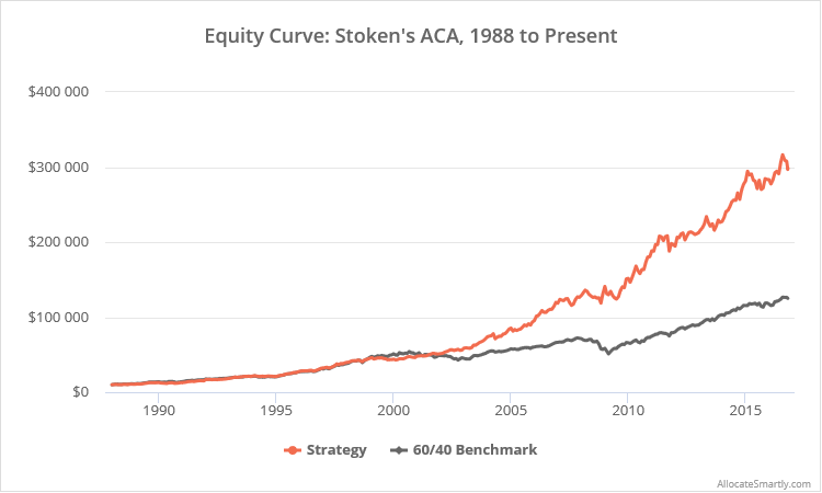
Figure 2 - ACA portfolio performance
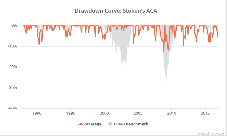
Figure 3 - ACA portfolio drawdown
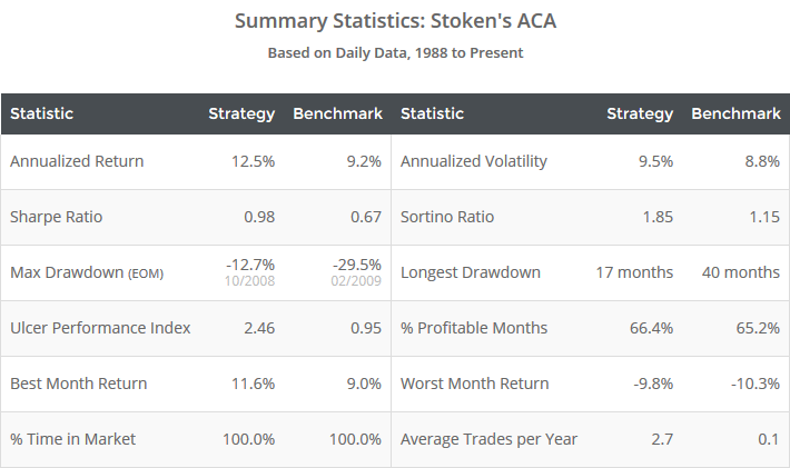
Figure 4 - ACA strategy statistics
Here we can see Stoken's ACA strategy compared against a simple 60/40 bonds/stocks portfolio over the period of roughly 30 years. As we can see ACA does better in terms of annualized return, Sharpe ratio, max drawdown and longest drawdown.
If you think 12.5% a year on average is not too much - think about compound interest. The "magic" of compound interest would allow you to multiply your investment 10 folds over the period of the last 20 years with this average return. Not too bad, is it?
Doublecheck
Now following the trust but verify mindset how about checking these statistics manually using Yahoo Finance data and Python open-source data-science tools?
As long as we're using Yahoo Finance ETF prices data we are limited to go only as far as 2004-11-18 when the GLD ETF started to trade - all other ETFs that we became available earlier but many around the same period.
The full Python code and results are available on Github. So here we only share strategy evaluation results and thoughts about it.
First, we have:
Annualized return is: 13.23%
over the period of 17.11 years
from 2004-11-18 to 2021-12-28
Compared to Allocate Smartly this is slightly higher. This is maybe due to slight differences in strategy implementation itself. Or how we tread data - e.g. our test doesn't use adjusted prices (those including historical dividends payout) but instead account for it explicitly using historical dividends information.
Another possible option is we're testing on a different time period, so annualized return which is the average return per annum - may differ.
Net let us take a look at drawdown analysis.
 Figure 5 - Manual drawdown analysis
Annualized volatility 10.91%
Sharpe ratio 0.94
Longest drawdown: 427 days, 14 months
From 2018-01-24 to 2019-03-27
Max drawdown -18.17% on 2020-03-19
Allocate Smartly looks at changes month-by-month and our analysis is day-by-day - which is more precise (higher resolution). Thus our volatility is higher (10.91% vs 9.5%) and so our max drawdown (-18.17% vs -12.7%). That is a pretty big difference to be underestimated by the Allocate Smartly backtest.
Also, the max drawdown valuation reached in 2020 according to our test and Allocate Smartly tells us it was in 2008. Again due to the same reason as above.
Our test's longest drawdown is shorter (14 months vs 17 months). But we tested on a shorter time period and we do not know on which period Allocate Smartly found their result (could be before 2004).
As to Sharpe ratio - it varies greatly depending on which risk-free rate \(R_f\) we choose for the formula, but both backtests show it's close to one. Which is a good value.
In our case we put \(R_f = 3.0\) the rate was not higher than that during the last five years according to LIBOR data.
Live test
The author is testing the strategy live since 2021-07-21 and till today 2021-12-29 the strategy yielded 6.64%. That result matches the backtest results over the same period quite closely.
Conclusions
We have learned that TAA investing strategies can help with reducing the risk without sacrificing profits too much.
Any backtest results are not set in stone. They may differ a lot depending on the used methodology. To they should have been taken with a bit of salt.
Basic tools for assessing portfolio risks are historical annualized volatility, max/longest drawdown and Sharpe ratio.
Python has a very nice free tooling for evaluating these metrics for your own investment strategy.
References
https://en.wikipedia.org/wiki/Variance
https://alf.katlex.com/blog/choosing-proper-etfs
https://alf.katlex.com/blog/king-of-hedge-funds-ray-dalio-advises-passive-investments
https://www.optimizedportfolio.com/all-weather-portfolio/
https://www.amazon.com/Survival-Fittest-Investors-Evolution-Portfolio-ebook/dp/B0076VLJ9W
https://www.investopedia.com/terms/s/sharperatio.asp
https://allocatesmartly.com/stokens-active-combined-asset-strategy
https://alf.katlex.com/blog/compound-interest-what-is-it-and-how-it-works
https://gist.github.com/alun/85fbc0d865a1bb5ac297d509cf3845f3